 RosyandBo.com Trusted Information and Education News Media
\(\newcommand{\Volume}{\mathrm{Volume}} \newcommand{\xLow}{\mathrm{xLow}} \newcommand{\xHigh}{\mathrm{xHigh}} \newcommand{\Mcost}{\operatorname{Marginal Cost}} \newcommand{\cost}{\operatorname{Cost}} \newcommand{\Mrev}{\operatorname{Marginal Acquirement}} \newcommand{\acquirement}{\operatorname{Acquirement}} \newcommand{\turn a profit}{\operatorname{Turn a profit}} \newcommand{\Mprofit}{\operatorname{Marginal Profit}} \newcommand{\Pprofit}{\operatorname{Predicted Profit}} \newcommand{\price}{\operatorname{Price}} \newcommand{\Dprice}{\operatorname{Demand Price}} \newcommand{\Pprice}{\operatorname{Purchase Toll}} \newcommand{\Sprice}{\operatorname{Supply Toll}} \newcommand{\marginal}{\operatorname{Marginal}\,} \newcommand{\linear}{\operatorname{Linear}\,} \newcommand{\abs}[i]{\left\lvert #ane\right\rvert} \newcommand{\quantity}{\mathrm{Quantity}} \newcommand{\AnnualCost}{\operatorname{Annual Toll}} \newcommand{\AnnualExpense}{\operatorname{Annual Expense}} \newcommand{\RepairFactor}{\mathrm{Repair Factor}} \newcommand{\Sales}{\operatorname{Sales}} \newcommand{\prediction}{\operatorname{prediction}} \newcommand{\FutureValue}{\operatorname{Future Value}} \newcommand{\demand}{\operatorname{Demand}} \newcommand{\val}{\operatorname{Value}} \newcommand{\raw}{\mathrm{raw}} \newcommand{\gizmos}{\operatorname{gizmos}} \newcommand{\intermediate}{\mathrm{intermediate}} \newcommand{\tax}{\operatorname{taxation}} \newcommand{\FaceValue}{\operatorname{Face up Value}} \newcommand{\rate}{\mathrm{rate}} \newcommand{\years}{\mathrm{years}} \newcommand{\expense}{\operatorname{expense}} \newcommand{\FutureAmount}{\operatorname{FutureAmount}} \newcommand{\InitialDeposit}{\mathrm{InitialDeposit}} \newcommand{\ppy}{\mathrm{ppy}} \newcommand{\PresentAmount}{\operatorname{PresentAmount}} \newcommand{\PriceGizmo}{\mathrm{PriceGizmos}} \newcommand{\QuantityGizmo}{\mathrm{QuantityGizmos}} \newcommand{\QuantityGadget}{\mathrm{QuantityGadgets}} \newcommand{\QuantityWidget}{\mathrm{QuantityWidgets}} \newcommand{\PriceWidget}{\mathrm{PriceWidgets}} \newcommand{\PriceGadget}{\mathrm{PriceGadgets}} \newcommand{\QW}{\mathrm{QW}} \newcommand{\QG}{\mathrm{QG}} \newcommand{\Prisoner of war}{\mathrm{Pow}} \newcommand{\PG}{\mathrm{PG}} \newcommand{\Product}{\operatorname{Production}} \newcommand{\Labor}{\mathrm{Labor}} \newcommand{\Capital}{\mathrm{Capital}} \newcommand{\Linear}{\operatorname{Linear}\,} \newcommand{\PriceX}{\mathrm{PriceX}} \newcommand{\PriceY}{\mathrm{PriceY}} \newcommand{\predicted}{\operatorname{predicted}} \newcommand{\Time}{\mathrm{time}} \newcommand{\TotalAmount}{\operatorname{TotalAmount}} \newcommand{\TotalValue}{\operatorname{TotalValue}} \newcommand{\CashAmount}{\mathrm{CashAmount}} \newcommand{\DepositAmount}{\mathrm{DepositAmount}} \newcommand{\AvailableTrees}{\operatorname{AvailableTrees}} \newcommand{\Capacity}{\mathrm{Capacity}} \newcommand{\Corporeality}{\operatorname{Amount}} \newcommand{\InitialAmount}{\mathrm{InitialAmount}} \newcommand{\InvestmentAmount}{\mathrm{InvestmentAmount}} \newcommand{\Return}{\operatorname{Return}} \newcommand{\SD}{\mathrm{SD}} \newcommand{\Antideriv}{\operatorname{Antideriv}} \newcommand{\MC}{\operatorname{MC}} \newcommand{\MP}{\operatorname{MP}} \newcommand{\MR}{\operatorname{MR}} \newcommand{\CDFf}{\operatorname{CDFf}} \newcommand{\Main}{\operatorname{Primary}} \newcommand{\ProducerSurplus}{\mathrm{ProducerSurplus}} \newcommand{\ConsumerSurplus}{\mathrm{ConsumerSurplus}} \newcommand{\TotalSocialGain}{\mathrm{TotalSocialGain}} \newcommand{\Elasticity}{\operatorname{Elasticity}} \newcommand{\lt}{<} \newcommand{\gt}{>} \newcommand{\amp}{&} \)
Link to unworked set of worksheets used in this department 1
Link to worksheets used in this section 2
Equally we mentioned in the previous chapter, many functions are locally linear, so if we restrict the domain the office will announced linear. Thus nosotros frequently start with linear models when trying to understand a situation. In this section we look at the concepts of supply and demand and market equilibrium. For our examples in this department nosotros will assume that the functions are linear in the range we care nigh.
Subsection
ii.ane.1
Supply and Demand and Market Equilibrium
The normal laws of supply and demand assume we are in a market with many producers and consumers, operating independently, all of them looking out for their own all-time interests. We expect that when the price goes up, more producers are willing to sell but fewer consumers are willing to buy. Conversely, when the price goes down, fewer producers are willing to sell but more consumers are willing to buy.
Consider the instance of gasoline prices. Dissimilar prices will brand some areas of exploration and production profitable or not profitable. When prices become up, new wells become drilled. If prices go down besides far, stripper wells end beingness profitable and are shut down. From the consumer side, when prices become up, more people await at mass transit or getting a more fuel-efficient vehicle. When prices go down, information technology is easier to think near a road trip.
The
constabulary of supply
looks at the economy from the supplier’due south point of view. Price and quantity bachelor for sale always motility in the same management. If the price goes upward we can assume that all the former suppliers are still willing to sell at the higher price, but some more than suppliers may enter the market. If the price goes down, no new suppliers will enter the market, and some old suppliers may leave the market. For a linear model:
\brainstorm{equation*} \text{slope of supply curve} = \frac{\text{change in price}}{\text{change in quantity supplied}} = \frac{\Delta p}{\Delta q} \gt 0\text{.} \cease{equation*}
The
law of demand
looks at the economic system from the consumer’due south point of view. Price and quantity available for sale always move in the reverse direction. If the cost goes downward we can assume that all the quondam consumers are nevertheless willing to buy at the lower price, but some more consumers may enter the market. If the cost goes upwardly, no new consumers will enter the market, and some old consumers may get out the market. For a linear model:
\brainstorm{equation*} \text{gradient of demand curve} = \frac{\text{modify in cost}}{\text{change in quantity demanded}}= \frac{\Delta p}{\Delta q} \lt 0\text{.} \end{equation*}
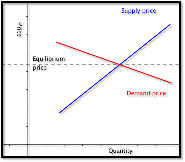
When we look at a graph of the supply price graph and the need price graph on the same graph, we know the supply curve goes up as nosotros become left to right, while the demand curve goes down. From the properties of lines nosotros know at that place is a single point where such a pair of lines can intersect. It is at the point where the amount of goods offered for a cost equals the corporeality of goods desired for the same price.
-
This intersection of the supply and the demand functions is called the point of
market equilibrium, or
equilibrium betoken. -
The cost at this indicate is referred to equally the
equilibrium price. -
The standard economic theory says that a free and open market will naturally settle on the equilibrium price.
Example
2.1.i
.
Starting With Formulas.
ii.1.2.
Video presentation of this example
Suppose
\(q\)
denotes quantity, and the supply price for widgets is given by
\begin{equation*} \Sprice =\$half-dozen+\frac{q}{100}\text{.} \cease{equation*}
We are too told the demand cost is given by
\begin{equation*} \Dprice=\$xviii-\frac{2q}{100}\text{.} \end{equation*}
Find the equilibrium cost and quantity.
Solution
i
.
Solution (a)
We have started with an example that we can do past basic algebra without whatsoever technology. Subtracting the two equations, we see that
\begin{equation*} 0=\$12-\frac{3q}{100}\text{.} \cease{equation*}
Some straightforward algebra shows that the equilibrium quantity is 400. Substituting back into either equation gives an equilibrium price of $10.
Solution
2
.
Solution (b)
While nosotros can do this case by hand, we besides want to use it to set up upward a solution with Excel, since nosotros may want help on problems where the numbers are not equally nice. Our plan is to use Goal Seek to find the intersection. Nosotros need a cell where we can solve the problem by forcing the cell to take a value of zero.
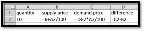
When cell
D2
is zero, the supply price will be the same every bit the demand price. Nosotros now invoke Goal Seek.
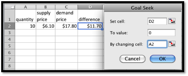
Equally expected, it finds equilibrium when
\(q=400\text{.}\)
We need to exercise a bit more work when we are simply given data points and need to find the supply and demand curves.
Example
two.1.3
.
Starting With Information.
ii.1.4.
Video presentation of this example
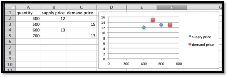
My market information indicates customers volition buy 700 gizmos if they are priced at $13 each. If the price rises to $15, they volition only purchase 500. If the toll is $12 a unit of measurement, the producers volition make 400 gizmos. If the toll rises to $thirteen, they volition produce 600 gizmos. Assume that the supply and demand curves are linear for between 300 and 1000 gizmos. Detect the equilibrium indicate for the gizmo market.
Solution
.
Nosotros start by making a chart for the values given. We add a scatterplot and then that we tin see the values.
Side by side nosotros add linear trendlines for both the supply and demand. We select the option to show the equations.
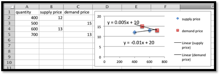
The projected equations are:
\brainstorm{marshal*} \Sprice\amp =0.005*\quantity+ten\\ \\Dprice\amp =-0.01*\quantity+20\text{.} \end{align*}
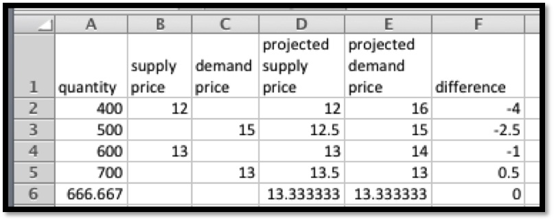
We ready up columns for the projected supply and demand curves. We too add a column for the difference so that we tin can apply Goal seek to find the equilibrium point.
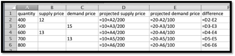
It is then straightforward to see that the equilibrium quantity is 666.67 and the equilibrium cost is $thirteen.33.
There is ane more detail worth noting from this final instance. Depending on the units used, the gradient can be very shut to zilch. If nosotros are selling tens of millions of units for a toll under a dollar, the change in price of a penny may correspond to a modify in quantity of several thousand. Make sure to include enough digits for your equation to be meaningful.
Example
2.1.5
.
Computing Sales.
ii.i.half dozen.
Video presentation of this case
We have obtained the following information for sales of gizmos in our location.
| quantity | 653 | 762 | 847 | 943 | 1050 | 1130 | 1260 |
| Supply cost | 5.52 | half dozen.20 | 6.85 | 7.48 | |||
| Demand price | half-dozen.68 | 6.fifty | half-dozen.38 | six.31 |
Assume the supply and demand curves are linear for quantities between 600 and 1300. Notice the best fitting lines for the supply and need functions. Find the equilibrium bespeak. Brand a chart listing how many we can sell for $6.40 and $6.60. Remember that sales volition exist the minimum of the supply and the demand.
Solution
.
We start by putting the data into a spreadsheet and finding the best fitting lines. We select the selection to show the equations in the chart.
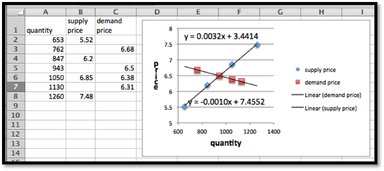
The supply and demand functions are:
\begin{align*} \Sprice \amp =.0032*\quantity+3.44\\ \Dprice \amp =-0.0010*\quantity+7.46\text{.} \terminate{align*}
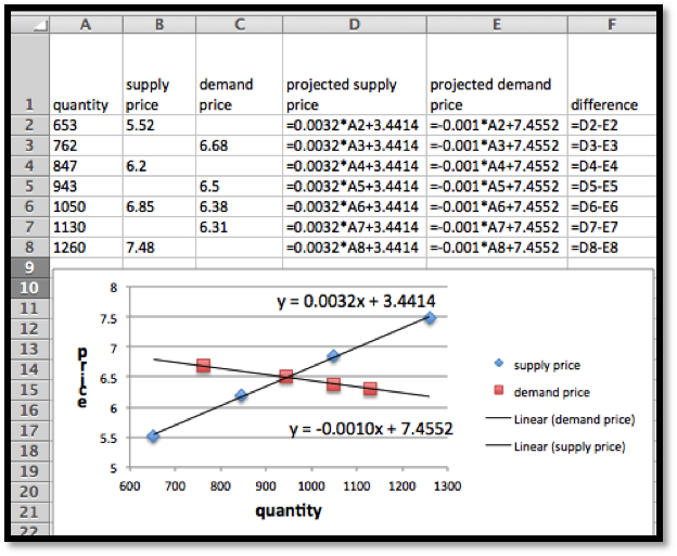
We add columns for the projected supply and demand prices, using the equations obtained from the best fitting lines. We also add a column, and compute the divergence of the supply and demand functions. We tin can now utilise goal seek to solve the trouble.
We now use Goal Seek to find the equilibrium bespeak.
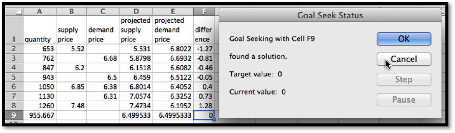
At equilibrium we sell 956 gizmos at $half dozen.50. To discover sales at $half-dozen.40 and $six.threescore, we utilise Goal Seek to get those values at both supply and demand prices.
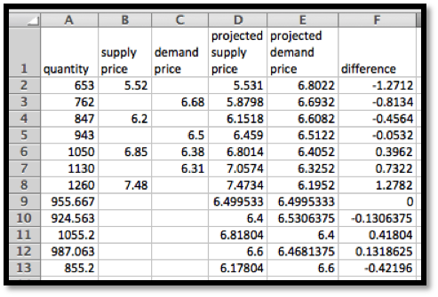
We see that we can sell 1055 gizmos at $6.40, simply can just obtain 925. Thus our sales at $half dozen.40 will exist 925. At $6.lx we tin obtain 987 gizmos, just tin merely sell 855. Thus our sales at $six.60 will exist 855. We can eliminate a step in this process if nosotros recollect that below equilibrium price the constraint is supply, while above equilibrium cost the constraint will be demand.
Exercises
2.i.ii
Exercises 2.1 Equilibrium Problems
Do Group.
Given the equations of the supply and demand curves:
-
Evaluate the curves at
\(q_0\text{.}\) -
Find the market equilibrium.
1.
Given
\(\Sprice=3 \quantity+10\)
and
\(\Dprice=-2 \quantity+30\text{,}\)
with
\(q_0=6\text{.}\)
Solution
.
-
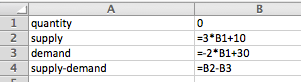
Entries in the cells before quick make full
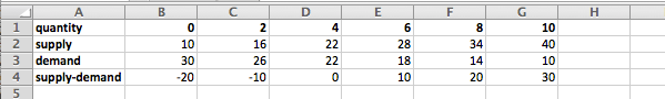
Table with quantities ranging from 0 to 10
From the table we meet that at
\(q_0=vi\)
the supply price is $28 and the demand price is $18. -
The market equilibrium happened to show up without requiring any more than work. The equilibrium occurs when
\(q = iv\)
and the price is $22.If we had not seen the equilibrium in the tabular array, nosotros should graph the table and determine what values of
\(q\)
nosotros should look at. Later adjusting the tabular array we can utilize Goal Seek to find the equilibrium signal: Solve\(\text{supply}-\text{demand}=0.\)
2.
Given
\(p_s=two q+xx\)
and
\(p_d=- q+200\text{,}\)
with
\(q_0=40\text{.}\)
3.
Given
\(\Sprice=.ii q+157.3\)
and
\(\Dprice=-0.01 q+3468.nine\text{,}\)
with
\(q_0=6000\text{.}\)
Solution
.
-
The initial entries:
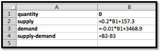
Initial attempt at the data includes the quantity 6000 (to answer part a)
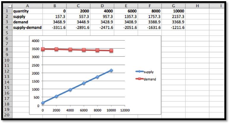
When
\(q = 6000\)
we have that the supply price is $1357.thirty and the demand price is $3408.90. -
The market equilibrium is outside the range that we tested. The graph indicates that the equilibrium (the intersection point) is to the correct of the values nosotros checked. Let’due south redo the table with
\(q\)
between 0 and xx,000. The increments are a matter of preference. In this example nosotros will use steps of 4000. The graph shows that the intersection point is somewhere between
\(q = 12,000\)
and
\(xvi,000\text{.}\)
The table shows it’south close to
\(q = 16,000\text{.}\)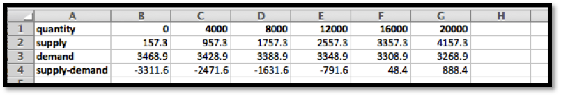
We employ Goal Seek to determine the actual equilibrium point.
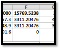
Goal Seek shows that the equilibrium point is at
\(q = 15770\)
with a toll of $3311.20
4.
Given
\(p_s=0.0035 q+23\)
and
\(p_d=-0.0027 q+463\text{,}\)
with
\(q_0=46,798\text{.}\)
v.
I am given
\(p=-2 q+100\)
and
\(p=iii q-30\text{,}\)
every bit my supply and demand curves, but am not told which is which. Decide which curve is the supply curve and explain how you did it. What limits can you put on the domain of the supply and demand functions?
Solution
.
The supply function is always increasing (positive gradient) and the demand office is always decreasing (negative gradient), so we have:
\begin{marshal*} \text{demand: } p \amp =-2 q+100\\ \text{supply: } p \amp =3 q-30\text{.} \end{align*}
We wait both functions to be positive, because negative prices would indicate we would take to actually requite people money to take our product off our hands!
\begin{align*} -2 q+100\gt 0 \amp \text{ implies } q\lt 50\\ 3 q-30\gt 0 \amp \text{ implies } q\gt ten\text{.} \end{align*}
So we should but consider quantities betwixt 10 and 50.
Exercise Group.
For Exercise ii.i.2.6–2.1.2.9, given the supply and need information:
-
Discover equations of the supply and demand curves, assuming they are both linear.
-
Find the market equilibrium.
6.
Given supply and demand information:
| quantity | l | 100 |
| Supply price | iv | ten |
| Need toll | ix | five |
7.
Given supply and demand data:
| quantity | 60 | 70 | 90 | 100 |
| Supply price | 14 | 20 | ||
| Demand price | 19 | 16 |
Solution
.
-
Nosotros start by using trendlines to discover the linear model functions.
In one case we take the function we create a second tabular array using the functions instead of the initial data. The equations were edited to indicate which one is the supply and which one is the demand function.
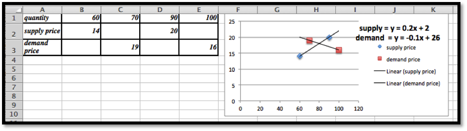
-
The 2nd tabular array will be ready to give united states of america the supply, demand and the supply − demand so we can utilize Goal Seek to find the market equilibrium.
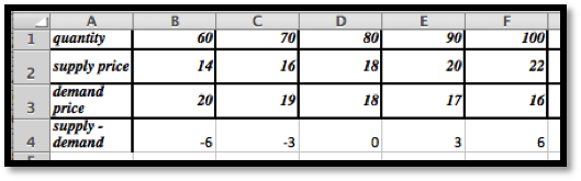
The market equilibrium occurs at
\(q = fourscore\)
with a cost of $xviii. (No Goal Seek required in this instance.)
8.
Given supply and demand data:
| quantity | 4356 | 4792 | 6503 | 7038 |
| Supply price | $ane.00 | $i.15 | ||
| Demand price | $i.10 | $.98 |
ix.
Given supply and demand data:
| quantity | 5378 | 7984 | 8352 |
| Supply price | $8.00 | $nine.50 | |
| Demand price | $12.00 | $10.00 |
Solution
.
-
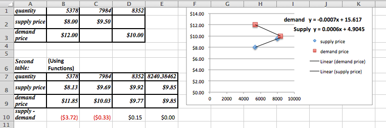
The supply and demand functions are:
\begin{align*} \Sprice (q) \amp = 0.0006 q+four.9045\\ \Dprice (q) \amp = -0.0007 q+xv.017\text{.} \end{align*}
These decimal approximations innovate a bit of an error: note the divergence between the recorded prices and the ones predicted past the model.
-
To notice the market equilibrium the cavalcade for
\(q = 8352\)
was copied and used to discover the equilibrium indicate. Note that Goal Seek simply works if the entries in the cells are formulas! The equilibrium is at
\(q = 8240\text{,}\)
with a price of $9.85. -
The projected prices are:
-
Supply cost of $9.92 when
\(q = 8352\) -
Demand price of $10.03 when
\(q = 7984\)
-
Exercise Group.
For Practice 2.1.ii.10–2.1.2.12, given the supply and demand data:
-
Find equations of the supply and demand curves, assuming they are both linear.
-
Find the market equilibrium.
-
Find the projected supply and need prices for the extra quantities given.
10.
Given the supply and demand information:
| quantity | 100 | 120 | 140 | 160 | 180 | 155 |
| Supply toll | 10.v | 11.8 | 13.9 | 16.3 | 17.5 | |
| Demand price | 21.3 | 18.1 | fourteen.7 | 12.iii | 8.half-dozen |
11.
Given the supply and demand information:
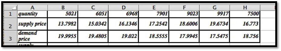
| quantity | 5021 | 6051 | 6968 | 7901 | 9023 | 9917 | 7500 |
| Supply price | 13.18 | 16.76 | 17.89 | 19.32 | |||
| Demand price | 19.69 | 18.78 | xviii.05 | 17.61 |
Solution
.
-
For this problem the trendlines are truly models and will find the all-time fit curve.
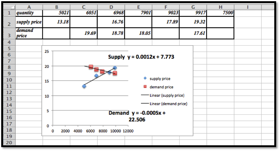
To be able to apply Goal Seek we do demand a table generated by formulas, so we use the trendline equations:
\begin{marshal*} \Sprice \amp = 0.0012 x+7.773\\ \Dprice \amp = -0.0005 x+22.506\text{.} \end{align*}
-
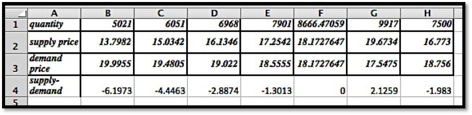
The market equilibrium takes place at
\(q = 8666.five\)
with a cost of $ 18.17. -
The projected prices are
12.
Given the supply and demand data:
| quantity | 3160 | 3615 | 4092 | 4462 | 4837 | 5261 | 5579 | 6000 |
| Supply price | 20.54 | xx.70 | 22.37 | 22.43 | ||||
| Need toll | 25.31 | 18.91 | 17.04 | 14.37 |
mathstat.slu.edu/~may/ExcelCalculus/external/Examples/Department-two-ane-Examples-unworked.xlsx
mathstat.slu.edu/~may/ExcelCalculus/external/Examples/Section-2-1-Examples.xlsx
Source: https://mathstat.slu.edu/~may/ExcelCalculus/sec-2-1-MarketEquilibriumProblems.html